TDGL Simulation

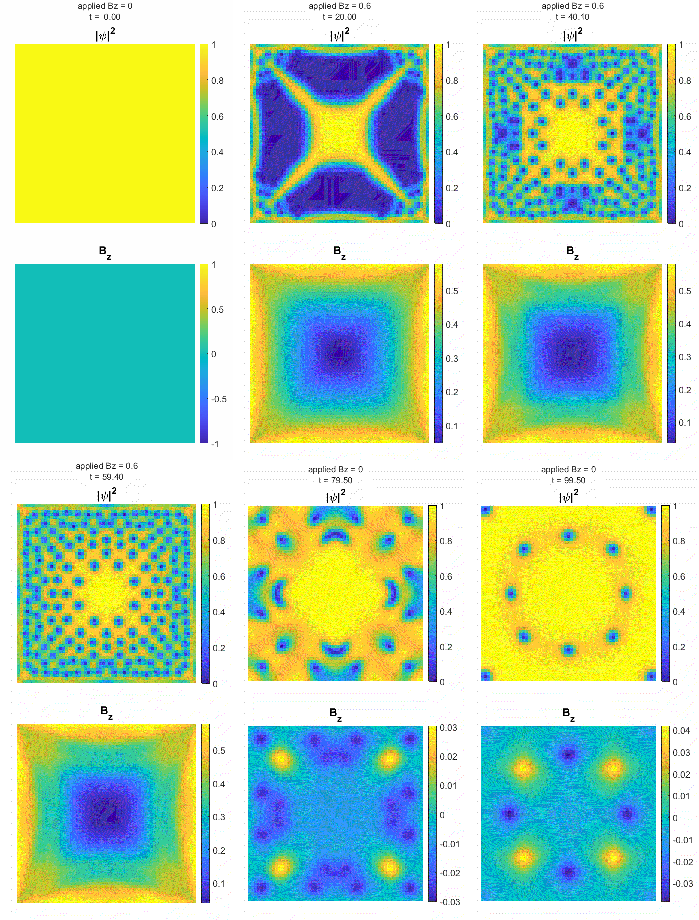
A 3D solver for the time-dependent Ginzburg–Landau equations, used to study vortex and phase dynamics in type-II superconductors. The order parameter ψ and the gauge field live on a structured finite-difference grid, with A stored as link variables (Peierls phases) on the edges so that gauge invariance and flux quantisation hold exactly on the lattice rather than approximately.

\frac{\partial \psi}{\partial t} = (\nabla - i\mathbf{A})^2 \psi + (1 - |\psi|^2)\,\psi

\frac{\partial \mathbf{A}}{\partial t} = \kappa^2 \nabla \times (\nabla \times \mathbf{A}) - \mathrm{Im}\!\left[\psi^* (\nabla - i\mathbf{A})\psi\right]

Everything is dimensionless: lengths in coherence lengths ξ, fields in $B_{c2}$ . Three numbers fix the normalisation — $\Phi_0 = 2\pi$ , $\lambda = \kappa$ (in ξ), and $H_{c2} = 1$ .

A 3×3 array of 4 µm holes

The coherence length fixes the grid spacing, but fabrication fixes the device, so a real hole array is a large simulation: nine 4 µm holes on an 8 µm pitch with an 8 µm buffer is 36 µm across, and at ξ = 150 nm that is 240 × 240 × 9 — 457 k nodes. At ξ = 50 nm it is 15 M nodes in 12 GB.

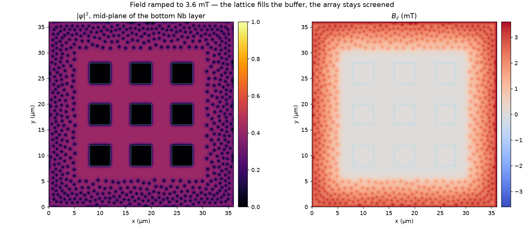
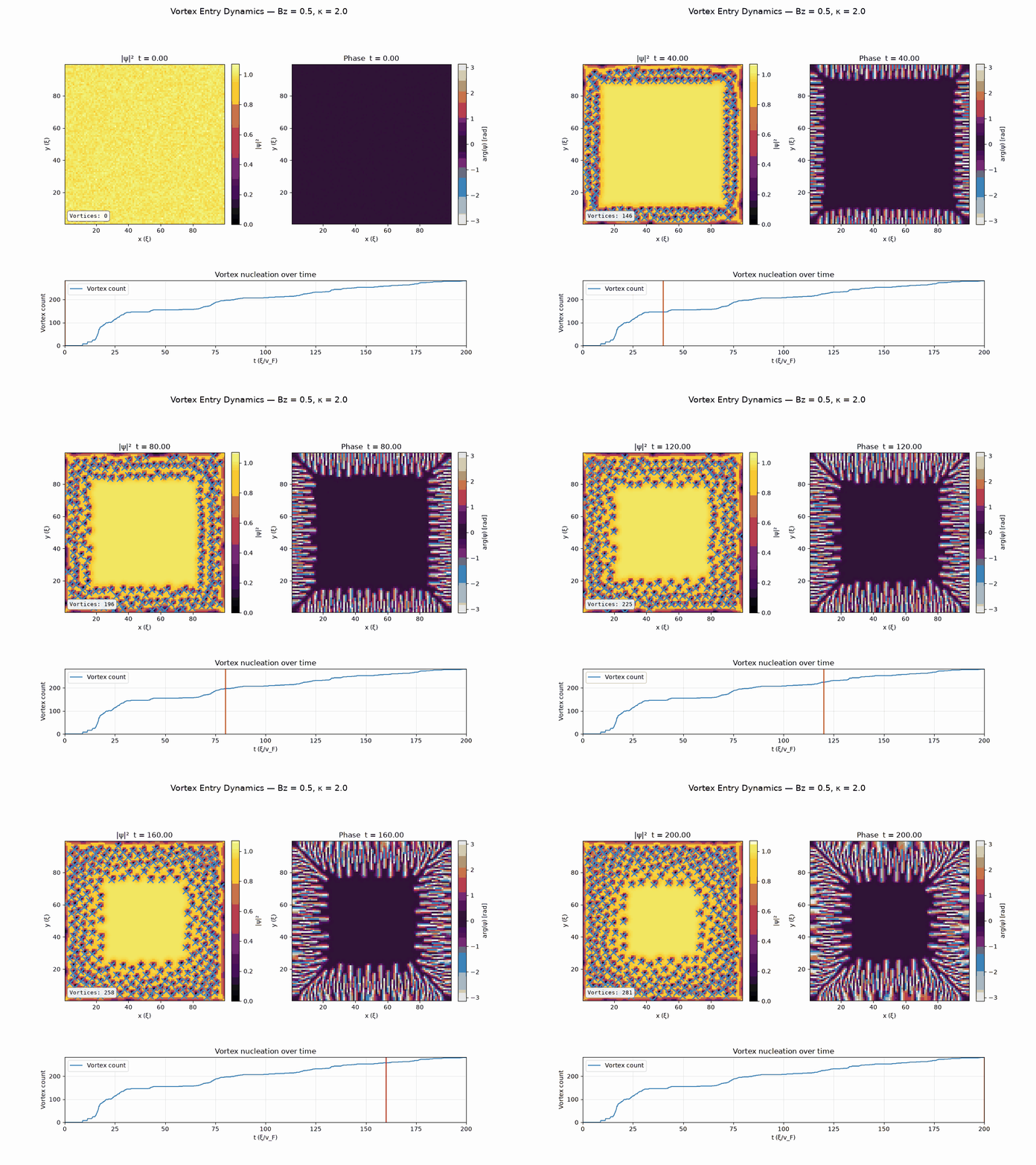
The obvious way to get flux into the holes does not work, and that is the interesting part. Ramping the field up, nothing enters until 3.15 mT — and just above that, hundreds of vortices enter at once. Held at 3.6 mT, 567 of them pack the buffer into a triangular lattice while the array stays fully Meissner-screened behind them: the flux front stalls at the array perimeter and never reaches a hole. There is no applied field at which this film holds one or two vortices in equilibrium; it holds none, or it holds hundreds.

Order parameter and Bz maps of a 3×3 hole array with the field ramped to 3.6 mT — Field ramped to 3.6 mT. The vortex lattice fills the buffer and stops at the array perimeter; the interior stays screened.

Field-cooling does what the experiment does. ψ grows from near zero with the field already on, so flux is trapped where it is rather than having to cross 8 µm of screening metal; the field then drops below the entry threshold and the state settles. Cooled at 4.0 mT and held at 2.0 mT, after 400 τ_GL: 3 vortices in the metal between the holes, 7 flux quanta trapped across the nine, with the rest of the flux in the buffer lattice. An independent run of the same protocol at another noise seed gives 2 and 6, with the census flat from t = 293 to t = 400 — so this is a settled state, not one realisation of the noise.

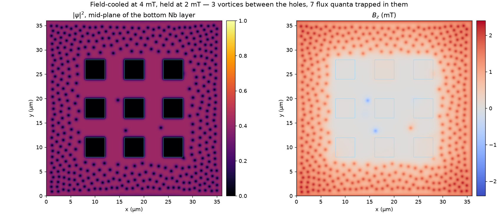
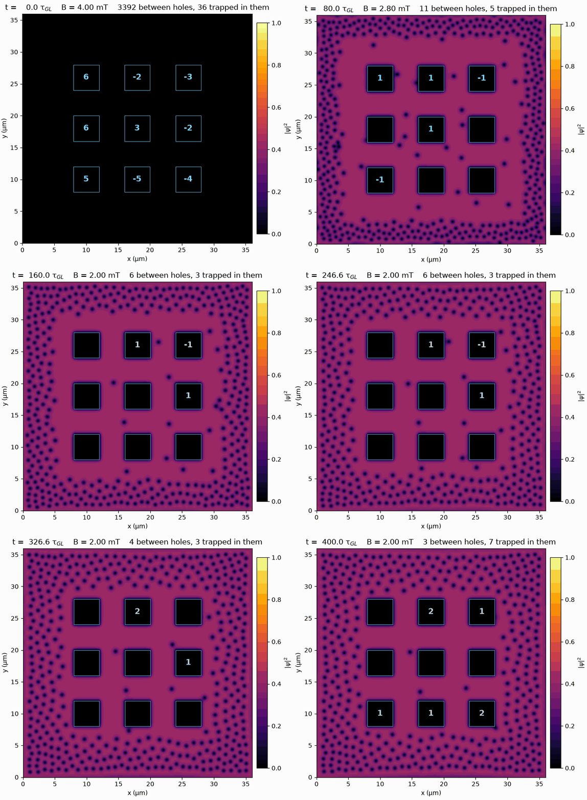
Field-cooled remanent state of the hole array: order parameter and Bz maps — Field-cooled at 4 mT, held at 2 mT. The array clears while the holes keep their fluxoid.

Animation of vortices entering and settling in the hole array, each hole labelled with its fluxoid — Getting there — each hole labelled with the fluxoid it holds.

The holes hold about one quantum each rather than the $B A/\Phi_0 \approx 19$ the applied field would suggest, and the $B_z$ map says why: 8 µm of buffer at λ = 300 nm leaves the array interior nearly field-free, so there is no local field there to support more. Per-hole occupancy is set by how well the surround screens, not by the applied field — which makes the buffer width and κ the levers.

A vortex in the film and a fluxoid in a hole are counted differently, because they are different things. The first is a core, found from the gauge-invariant phase winding around a plaquette; the second has no core to find and is read from the winding on a contour drawn in the metal around the hole, which is an exact integer however little field threads the opening.

Flux expulsion by an S/I/S ring

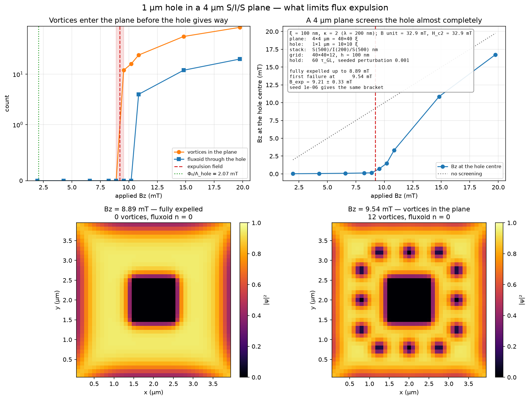
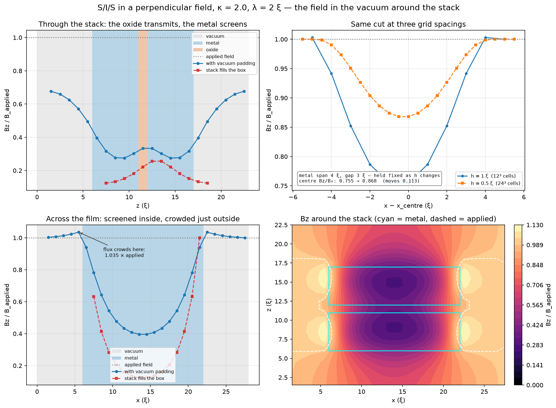
A 1 µm hole centred in a 4 µm S/I/S plane with 500 nm layers, at ξ = 100 nm — Nb near $T_c$ , where Ginzburg–Landau applies. The device expels flux completely — no vortices anywhere, zero fluxoid through the hole — up to 9.2 ± 0.3 mT.

What limits it is not the hole. A 4 µm plane is 20 λ across and screens so well that only 1.7% of the applied field reaches the hole (0.07 Φ₀ through it at the threshold), so the ring is nowhere near its fluxoid limit; vortices penetrate the 1.5 µm-wide arms first, and the hole does not admit a fluxoid until 10.9 mT. The device therefore beats the naive single-loop estimate $\Phi_0/A_\text{hole} = 2.07$ mT by more than a factor of four.

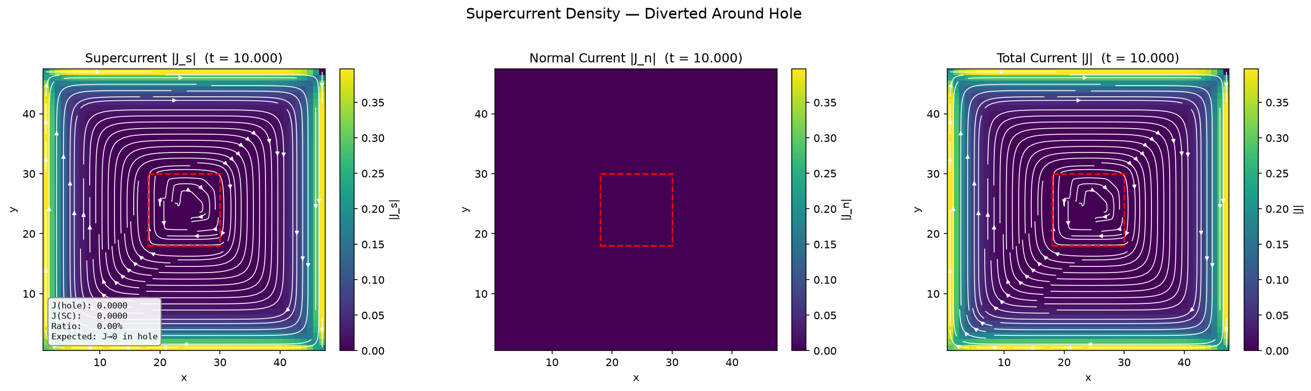
Four-panel figure: vortex and fluxoid counts against applied field, field at the hole centre, and order-parameter maps below and above threshold — Vortices enter the plane before the hole gives way. Click for full size.

Bz cuts through and across an S/I/S stack, and a Bz map of the field around it — S/I/S in a perpendicular field — the metal screens, the oxide transmits, and the expelled flux crowds into the vacuum beside the film.

Nucleation and screening currents

Animation of vortex nucleation: order parameter, phase, and a running vortex count — Vortices enter from the edges, interact, and settle into a steady population at Bz = 0.5.

Supercurrent, normal current and total current streamlines around a square hole — Supercurrent, normal current and total current around a square hole: J_s circulates around the hole and vanishes inside it.

Checks against exact solutions

Two limits of the coupled equations have closed-form solutions, and between them they exercise each equation on its own. Both comparisons have no fitted parameters, and both run at three grid spacings so the residual can be shown to be discretisation error rather than disagreement.

In the London limit (|ψ| = 1, so the ψ-equation drops out) a square with the field pinned on its boundary obeys $\nabla^2 B = B/\lambda^2$ , which has an exact Fourier solution. The solver matches it to rms 4.1e-3 · B₀ at h = 1 ξ, falling to 3.3e-4 at h = 0.25 ξ — observed order 1.82 in h. On the pinned boundary plaquettes, where the condition is Dirichlet and the solver should be exact rather than approximate, it agrees with the applied field to 6e-16.

At a pair-breaking wall (zero field, so the gauge field drops out) $\psi'' = -\psi + \psi^3$ gives $\tanh((x - x_0)/\sqrt{2})$ , with the offset $x_0$ fixed by matching to the insulator’s relaxation rather than fitted. The solver matches it to rms 5.0e-2 at h = 1 ξ, falling to 4.8e-3 at h = 0.25 ξ — observed order 1.69 in h. The √2 is the physics being checked: the Ginzburg–Landau healing length is √2 ξ, not ξ.

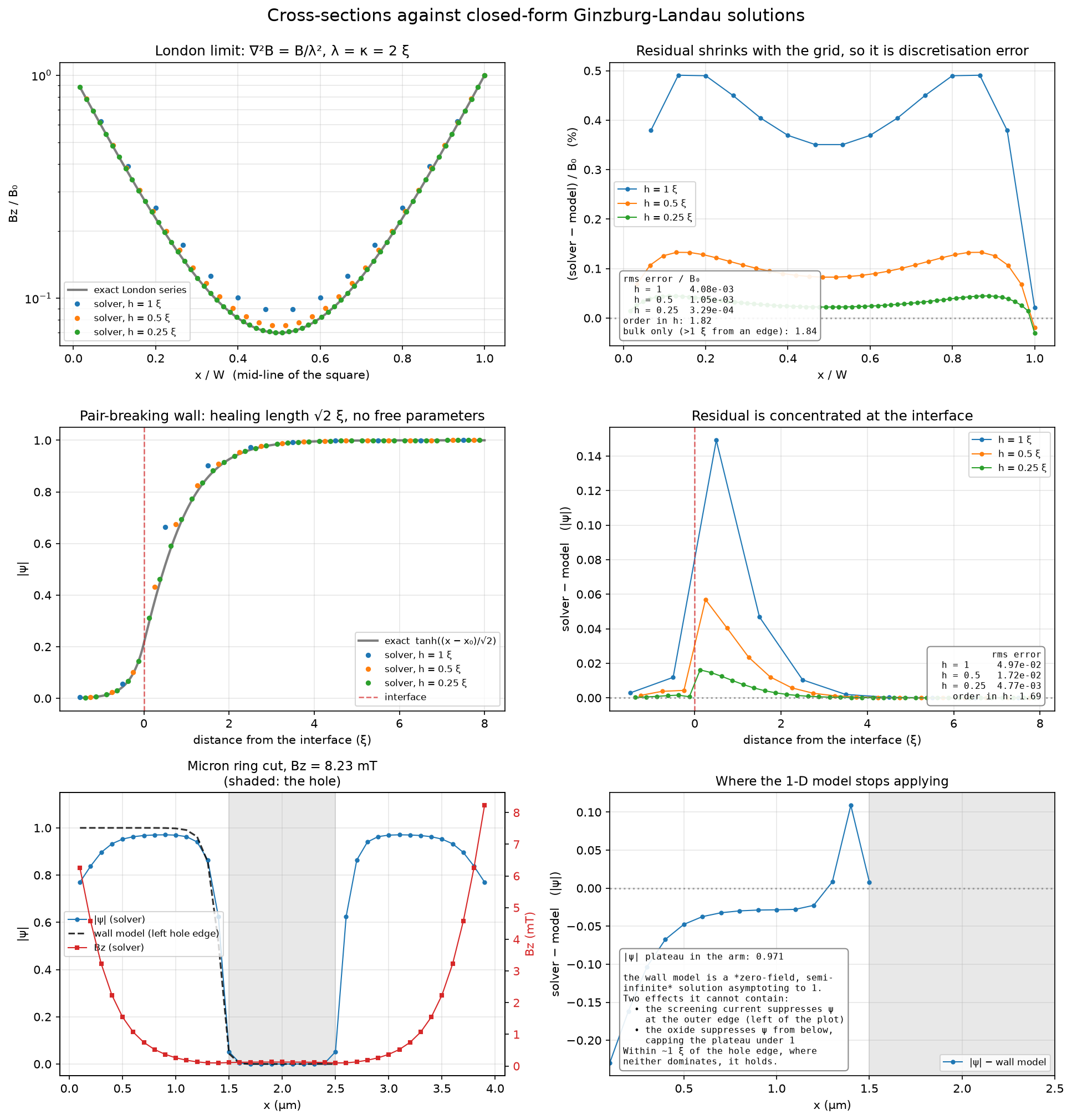
Six-panel comparison of solver cross-sections against closed-form London and pair-breaking-wall solutions, with residuals at three grid spacings — Cross-sections against closed-form solutions, with the residual at three grid spacings. The bottom row applies the same two models to the micron ring, where neither holds exactly, and says where each stops applying. Click for full size.

The 3D path is checked against the same exact solution: a problem with no z-dependence must be solved identically by the 2D and 3D codes, and it is — the field varies across z-slices by 2e-16 and differs from the 2D run by 2e-10. Altogether the verification suites record 294 physics checks — gauge covariance, ∇·B = 0, symmetry, fluxoid quantisation, the closed-form limits — each with its measured value, the value physics requires, and the tolerance allowed.

Scale

The device above is 1.8 M nodes at ξ = 100 nm, and it is the size that decides whether a study is an afternoon or a month. Measured on 4 cores, per unit of Ginzburg–Landau time, with forward Euler at 0.9 of the CFL limit:

ξ(T)	grid	interior nodes	s per τ_GL	peak RSS
150 nm	240 × 240 × 9	457 k	5.5	0.5 GB
100 nm	360 × 360 × 15	1.80 M	25.2	1.6 GB
70 nm	514 × 514 × 21	5.26 M	132	4.3 GB
50 nm	720 × 720 × 30	15.0 M	475	12.1 GB

All four were run, not extrapolated. Three knobs matter at that scale: a thread pool for the right-hand side (bandwidth-bound, so cores help — 3.1× on four), streaming frames to HDF5 as they are produced so memory holds one frame however long the run is, and single precision, which halves both the memory and the bandwidth the evaluation is limited by.

Use forward Euler. The implicit trapezoidal integrator costs roughly 8× more per unit simulated time on a grid this size: its Newton–GCR inner solve is unpreconditioned, so the Krylov iteration count grows about as fast as the step size it buys and the larger step never pays for itself.

Getting started

git clone https://github.com/omedeiro/nanowire_tdgl.git
cd nanowire_tdgl/packages/tdgl3d
pip install -e ".[dev]"
pytest

import tdgl3d

params = tdgl3d.SimulationParameters(
    Nx=20, Ny=20, Nz=4,
    hx=1.0, hy=1.0, hz=1.0,
    kappa=5.0,
)
field = tdgl3d.AppliedField(Bz=1.0, ramp=True, ramp_fraction=0.3)
device = tdgl3d.Device(params, applied_field=field)

solution = tdgl3d.solve(device, t_stop=10.0, dt=0.05, method="euler")

solution.plot_order_parameter(slice_z=2)

The hole-array figures are reproduced by packages/tdgl3d/examples/nb_hole_array.py, whose --dry-run prints the grid, the memory per frame and a wall-time estimate before you commit to a run. Every figure above is produced by a standalone script in docs/figures/.

MATLAB predecessor

The Python package is a rewrite of the 3D TDGL MATLAB code written for MIT 6.336 (Spring 2021), verified against it index for index.

TDGL order parameter and magnetic field time evolution — Time evolution of a type-II superconductor under a 0.6 mT applied field in the z-direction, turned off at t=65. Top: 2D color map of the order parameter. Bottom: 2D color map of the z-component of the magnetic field.

Rotating view of the |psi|^2 = 0.1 isosurface in a 3D film — The |ψ|² = 0.1 isosurface in a 3D film, from the same MATLAB code.

Source

github.com/omedeiro/nanowire_tdgl — the Python package. The original MATLAB is in github.com/omedeiro/simulation6336.