Bertrand's Paradox

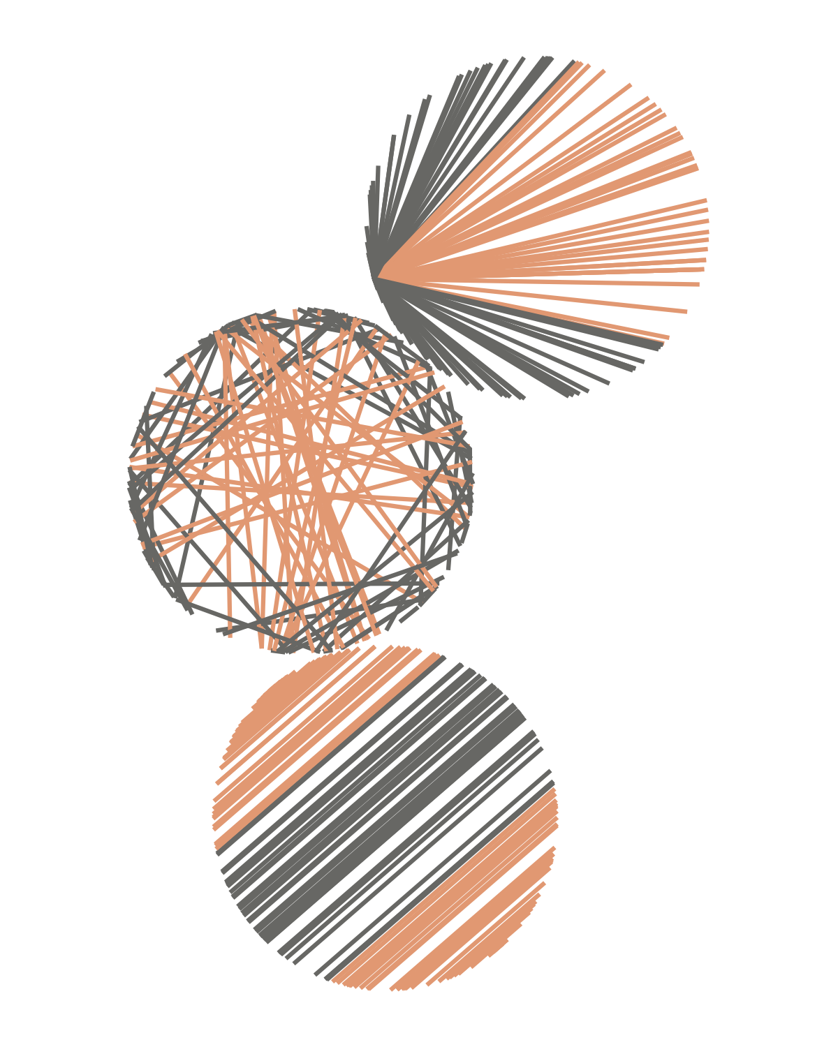
Joseph Bertrand set the problem in his Calcul des probabilités of 1889, and answered it three times. Draw a chord of a circle at random: what is the probability that it comes out longer than the side of the inscribed equilateral triangle? Three constructions, each a reasonable reading of “at random”, give $1/3$, $1/2$ and $1/4$ — and none of them is doing arithmetic wrong.

Pick a method and drag the slider; Run streams the sample in so the estimate can be watched settling.

The dashed triangle is the thing being compared against; chords longer than its side are drawn in the accent colour. Show → Midpoints replaces each chord with its own midpoint, which is where the methods separate most clearly, and adds the circle of half the radius that the midpoint has to fall inside. Compare all four puts them side by side. Expand fills the screen; Esc leaves it.

Push the count up and a pale disc appears in the middle of the bundle, exactly the triangle’s incircle. Nothing is being drawn there but the long chords: a chord at distance $p$ from the centre leaves the whole disc of radius $p$ untouched, so the only ones reaching inside radius $\tfrac12$ are the ones the question is counting.

One number, not two

Take the circle to have radius $1$. A chord is fixed by the foot of the perpendicular dropped onto it from the centre: a distance $p \in [0, 1]$ and a direction. Every method here treats directions alike, so the direction carries no information and the whole question rests on $p$. The chord’s length is

and the inscribed equilateral triangle has side $\sqrt3$, so

That is the entire geometry. A method is not a construction but a probability density on $p \in [0,1]$, and the answer it gives is the area of that density to the left of $\tfrac12$ — which is the shaded half of the strip under the circle, with the sampled histogram drawn against the exact curve.

Where the three answers come from

Two points on the circumference. Rotate so the first endpoint sits at angle $0$; the second is at $\theta$, uniform. Then $p = \lvert\cos(\theta/2)\rvert$, and with $u = \theta/2$ uniform on $[0, \pi)$ that is the arcsine law $f(p) = 2/\pi\sqrt{1-p^2}$, crowding both ends. The chord beats the triangle when $u \in (\pi/3, 2\pi/3)$ — a $120°$ arc out of $360°$, so $P = 1/3$.

A point along a random radius. Choose a radius, then a point uniformly along it, and take that point as the chord’s midpoint. Now $p$ is uniform by construction, $f(p) = 1$, and $P = 1/2$ needs no work at all.

A point anywhere in the disc. Choose the midpoint uniformly over the area. The midpoint of a long chord is one lying inside the circle of radius $\tfrac12$, so $P$ is the ratio of the areas, $(\tfrac12)^2 = 1/4$. In terms of $p$ the density is $f(p) = 2p$: there is simply more disc at large radius, which is what pushes the answer down.

The midpoint view shows all three at once. Uniform midpoints fill the disc evenly. Uniform $p$ along a radius makes the density go as $1/p$, so the same chords pile up at the centre. Uniform endpoints push them out to the rim.

A fourth, for the sake of the argument

Drop two points into the disc at random and extend the line through them. This one is not in Bertrand, but it is the least contrived way to get a chord out of a physical procedure, and it lands nowhere near the other three.

Pairs of interior points sitting on a given chord are not equally common: writing a pair as a line plus two positions $t_1, t_2$ along it, the area element picks up the Jacobian $\lvert t_1 - t_2\rvert$, which integrates over a chord of length $\ell$ to $\ell^3/3$. So this procedure samples lines with a weight of $\ell^3$, and

Long chords are wide targets, and cubing the length is a heavy thumb on the scale.

Every answer is available

Nothing stops at four. The family $f(p) = (\alpha+1)p^{\alpha}$ is a density on $[0,1]$ for any $\alpha > -1$, and it gives

which sweeps the whole open interval $(0,1)$ as $\alpha$ runs from $-1$ to $\infty$. Two of Bertrand’s own answers are already in there — $\alpha = 0$ gives $1/2$ and $\alpha = 1$ gives $1/4$ — and so is every other number you might want, including $0.99$. The question as posed does not have three answers. It has all of them, and stopping at three is a rhetorical choice rather than a mathematical one.

Fixing one endpoint changes nothing

The most common way to get this wrong — and what an earlier version of this page did in MATLAB — is to describe the second method as fix one endpoint and choose the other at random. That is not the radius construction. It is the first method with the rotation already applied: conditional on the first endpoint, the second is still uniform on the circle, so the chord is long exactly when it lands in the $120°$ arc opposite, and the answer is $1/3$ again. Nailing down one endpoint costs nothing, because the first method never used it. What makes the second method different is that the uniform variable is the midpoint’s distance from the centre, not a point on the circumference.

Jaynes and the well-posed problem

Edwin Jaynes’ answer, in “The Well-Posed Problem” (Foundations of Physics 3, 1973), is that the question is underspecified in a way that can be repaired rather than merely deplored. The problem says nothing about where the circle is or how large it is, so a solution that deserves to be called the solution should not depend on either: the same rule, applied to a circle shifted a little or shrunk a little, has to give the same distribution of chords. Invariance under translation and scaling turns out to force $f(p) = 1$, and with it $P = 1/2$.

The same measure arrives from integral geometry, where $dp\, d\varphi$ is the only measure on lines in the plane invariant under rigid motions, and Jaynes checked it in the least abstract way available by tossing broom straws at a circle drawn on the floor.

That settles the version of the question about a random line that happens to meet a circle. It does not make the other constructions wrong, because they are answers to other questions — about pairs of points on a rim, or about midpoints scattered over a disc — each of which is perfectly well posed once stated. The paradox is not about probability being ambiguous. It is about “at random” not being a specification.

Notes on the sampler

Sampling runs off a seeded generator rather than Math.random, and each method keeps its own stream. Raising the count therefore extends the sample instead of drawing an unrelated one: chords already on screen stay where they are and new ones appear among them, which is what makes the slider read as convergence rather than as a shuffle. Resample is the way to ask for a genuinely different draw. The running count of long chords is kept as a cumulative array, so the estimate at any prefix of the sample — every frame of Run — is a single lookup.

Each sample is stored as its two endpoints and its midpoint, and the chords are drawn in two batched paths, one per colour, rather than one path each. Opacity falls as the count rises so that four thousand chords read as shading rather than as a solid disc, and the histogram under the plot is normalised to a density so the bars and the exact curve share one vertical scale. The arcsine density is unbounded at $p = 1$, so that axis is clipped — which is why the endpoint method’s curve runs off the top of the strip near the rim.

Download the sampler source